Monday 26 October 2015

Saturn's Shifting Seasons from a Decade of Cassini Observations

Last year the Cassini spacecraft celebrated the end of a decade of exploration of the gas giant Saturn, yet another milestone in a mission that is finally set to end in a fiery plunge into Saturn’s atmosphere in September 2017.  When that time comes, Cassini will have been orbiting the ringed world for half of a Saturnian year, from perihelion to aphelion and from northern winter solstice to northern summer solstice.  Saturn’s 27-degree axial tilt subjects the atmosphere to seasonal shifts in sunlight over its 30-year orbit of the Sun.  The atmosphere responds to this changing solar energy deposition, generating hemispheric asymmetries in temperature, composition and cloud coverage that alter over time.  Large-scale circulation patterns move energy from one hemisphere to the other, and the associated meteorology and chemistry lead to changes in the soup of species that make up Saturn’s atmospheric composition. 

The unprecedented duration of Cassini’s reconnaissance of Saturn is allowing planetary scientists to study the implications of the shifting seasons for the first time.  Dr. Leigh Fletcher, Senior Research Fellow in RSPP and co-investigator on Cassini, has recently published a new study of Saturn’s shifting temperatures and composition from Cassini in the journal Icarus (Fletcher et al. 2016, Icarus 264, p137-159, http://arxiv.org/abs/1509.02281), using a thermal-infrared instrument called CIRS (the Composite Infrared Spectrometer).  By considering many thousands of spectra taken since 2004, Fletcher and colleagues were able to reconstruct Saturn’s changing climate in three dimensions – latitude, altitude and time – constructing the first ever movies of Saturn’s changing environmental conditions. 

The movies revealed the slow warming of Saturn’s northern hemisphere as it emerged from the darkness of polar winter into spring sunlight.  Air began sinking over Saturn’s northern polar region, carrying chemicals along with it so that these species (notably spin isomers of hydrogen and hydrocarbons produced by methane photochemistry) became enriched in the northern hemisphere as spring progressed.  Likewise, as Saturn’s autumnal hemisphere descended into winter darkness, the movies revealed the cooling and disappearance of a large warm seasonal vortex over Saturn’s south pole.   The results also showed that Saturn doesn’t respond instantaneously to the sunlight changes – the atmosphere has such a large thermal inertia that the coldest northern conditions are actually found in springtime rather than at winter solstice, lagging almost a season behind the solar insolation.

Zonal mean cross-sections of atmospheric temperatures before, during, and after the equinox of 2009, showing seasonal cooling in the autumnal southern hemisphere and warming in the springtime northern hemisphere.  These large-scale asymmetries are superimposed onto the belt/zone structure of cool zones and warmer belts that typify the atmospheres of Jupiter and Saturn.


Fletcher and colleagues used the movies to investigate the dynamical, meteorological and chemical consequences of the shifting seasons, including the ability of Saturn’s atmosphere to host planetary wave activity.  These waves, potentially launched into the stratosphere by powerful weather activity at deeper levels, can only propagate under certain atmospheric conditions.  One striking example of that was the intense springtime storm, which launched waves high into the overlying stratosphere in 2010-11.   These storms appear to happen once per year during spring or summer, but how these enormous storms might be linked to the seasonal cycle remains a topic of ongoing investigation.  Finally, the shifting temperature was shown to alter the atmospheric chemistry and the production of hazes.  These hazes are responsible for Saturn’s familiar ochre appearance, and were notably absent from Saturn’s blue northern hemisphere early in Cassini’s mission.  As the temperatures warmed, aerosol particles grew in size and Saturn’s ‘blues’ dissipated, providing a direct connection between Saturn’s shifting temperatures and the colours we can see in the clouds. 

These results form a part of a new book on Cassini’s discoveries on Saturn that will soon be available from Cambridge University Press.  Fletcher’s chapter on Saturn’s seasons is available as a preprint (http://arxiv.org/abs/1510.05690).

Monday 19 October 2015

Jupiter Weather Report: 2015/16 Apparition

[Work in Progress]

Jupiter will be intensely scrutinised over the next six or seven months to understand the state of the atmosphere immediately prior to the arrival of the Juno spacecraft in July 2016.  The spacecraft team hopes to use guidance from the citizen science record to target specific features of interest, from storms and plumes to large-scale changes in Jupiter's banded structure.  At the end of the last apparition, we were awaiting both an outbreak on the North Temperate Belt jetstream and an expansion event in the North Equatorial Belt.

Some of the first images of the apparition started to arrive in October 2015, and have once again been assembled into a glorious map by Marco Vedovato of the Italian Amateur Astronomers Planet Section.  He uses the WinJUPOS software tool to create global maps of Jupiter regularly during the apparition - his index of maps can be found here.

JUPOS map of Jupiter at the start of the 2015/16 apparition (October 15-18 2015).  Credit:  M. Vedovato.
South Tropical Domain:
The GRS remains extremely orange in colour, with chaotic activity in its northwestern wake region.

North Tropical Domain:
White Spot Z (WSZ) is still apparent on the ragged northern edge of the NEB near 19N, but a conspicuous new Red Spot can also be seen sat between the NTropZ and the NEB.  There are no signs yet of the NEB expansion event starting.

South Temperate Domain:
The chain of Anticyclonic White Ovals (AWOs) still persists in the South South Temperate Belt near 40S.

North Temperate Domain:
The northern barges on the North Temperate Belt (NTB) that were so prominent for much of the previous apparition are no longer quite so visible.

Tuesday 29 September 2015

Jupiter Weather Report: 2014/15 Apparition

In an earlier post, I described how the army of citizen scientists provide near-continuous updates on Jupiter's atmospheric phenomena, allowing the British Astronomical Association and others to provide regular digests on jovian weather and reasonable forecasts of what might be coming.  At the time of writing (September 2015) Jupiter is a few weeks past solar conjunction and ready to make it's reappearance in our dawn skies, so the 2014/15 apparition that was centred on the February 6th opposition (when Jupiter was at its biggest and brightest) is now over.  Scientists all over the world are preparing observing proposals for the next 2015/16 apparition on Earth-based observatories, which will be the final opportunity to characterise Jupiter's churning weather before the arrival of the Juno spacecraft on July 4th 2016.  For details of the nomenclature of Jupiter's belts and zones, please refer to my previous post.

From the amateur community, the first images of the apparition were uploaded to PVOL on August 31st 2014, and the last ones on July 31st 2015.  I'm indebted to Marco Vedovato of the Italian Amateur Astronomers Planet Section for using the WinJUPOS software tool to create global maps of Jupiter regularly during the apparition - his index of maps can be found here.   Further insights into Jupiter's complex goings-on have been provided by the wonderful Hubble Space Telescope's OPAL (Outer Planet Atmospheres Legacy) project, led by Amy Simon, Mike Wong and Glenn Orton. Hubble observations of Jupiter on January 19th 2015 are available here, and a new '4K movie' released by HST can be seen below.

Jupiter as observed on January 19th 2015 by the Hubble Space Telescope WFC3 instrument.  The findings of the new dataset are described by Simon et al., 2015, ApJ, 812, 55

Below I've provided links to some of Vedovato's JUPOS maps for various points during this apparition - they prefer having north to the bottom of the images as this is how Jupiter would really be seen through the eyepiece.  The following four images were taken between October 2014 and April 2015, and you can see the evolution of features by toggling between them (all should be credited to Marco Vedovato and the JUPOS team).


South Tropical Domain:  GRS Shrinkage has Slowed?

Jupiter's Great Red Spot, sat between the SEB and STropZ, has been steadily shrinking in east-west extent for many years (we've known this for a while, despite recent news reporting!).  A couple of years ago the community discovered that this shrinkage had gone through an unprecedented acceleration, with measurements by citizen scientists suggesting a longitudinal width of 13.6±0.7 degrees in 2013/14, down from 15.3±0.8 degrees in 2011/12.  In 2014/15 this longitudinal shrinkage seems to have stopped or slowed down, with the size being the same as last year - approximately 13.8±0.9 degrees longitude according to measurements by the JUPOS team (Vedovato et al. - see his charts here).  M. Jacquesson was able to use November 2014 images to measure the internal rotation of the GRS at approximately 3.8 days, consistent with values measured in the 2013/14 apparition.

Observations from the Hubble Space Telescope (Simon et al., 2015) captured some wonderful spiralling filamentary structure within the GRS core, and indicated that the core of the GRS remains just as orangey-red as it did in the previous 2013/14 apparition, consistent with the general appearance in the amateur imaging.  It has narrowed in latitudinal (north-south) extent too, implying a less severe interaction with the SEBs retrograde jet that flows around its northern periphery.

As for the rest of the South Equatorial Belt (SEB), it appears to be business as usual - lots of complex rifting in the turbulent wake to the northwest of the Great Red Spot, and no sign of any 'fading activity' such as that last witnessed in 2009/10, when the entire SEB whitened over.  It's really hard to predict these SEB whitening cycles, so who knows when the next might begin!

North Tropical Domain:  Waiting for an NEB Expansion:

North Equatorial Belt (NEB):  The width of this dark-red belt changes over time, having shrunk during 2013 with the disappearance of the dark, distinct brown barges on its northern edge.  At the end of the 2014/15 apparition it may be on the verge of expanding again (the last such event took place in 2012), meaning that those brown barges could reappear during the next apparition.  NEB broadening events have been occurring at 3-5 year intervals since 1988, so we might expect another in the next couple of years - observers will be waiting to see if such a dramatic change in the belt/zone structure happens next year.  One of the most conspicuous features is 'White Spot Z', a white oval right on the ragged northern edge of the NEB (near 17N) that had a more reddish tinge last apparition.  This white spot can also be seen in the Hubble imaging.

The OPAL images in January 2015 captured some fine-scale waves within the NEB near 16N, a type of structure known as a baroclinic wave, not seen in Jupiter imaging since the Voyager days.  This fine wave was superimposed on top of other NEB cloud features, including a chain of cyclones at the same latitude and whiter anticyclones on the northern edge of the NEB (the retrograde jet called the NEBn).

North Temperate Domain:  Brown Barges:

The Northern Temperate Domain last underwent an upheaval back in 2012, and the cloud structures in this region still appear complex 3 years on.  In particular, there are several cyclonic 'Brown Barges' on the North Temperate Belt (NTB) near 30N:  4-5 brown barges are now evident within the NTB and are extremely elongated in east-west extent.  John Rogers suggests that rifting during the previous apparition generated an extremely dark spot in the Northern Temperate Zone (NTZ), which lengthened to become a dark streak that somehow evolved into the extremely long barge that we see today.

In general though, there were no signs of large NTB outbreaks (plumes on the jets), which occur at approximately 5-year intervals - the next one is likely to occur in 2016 or 2017, right smack bang in the middle of the Juno mission.  The NTB might have been showing signs of fading, as it does just before an outbreak, but when Jupiter disappeared from view the NTB was still unchanged...

The amateur community caught the birth of a new Little Red Spot in December 2014, just to the north (32N) of the brown barges.  It can be seen in the Hubble imaging, below.  It started as a white spot interacting with other ovals (that didn't survive), becoming larger and fawn-coloured, before appearing brighter and redder in January 2015.

Annotated version of Hubble imaging in January 2015, showing structures at all latitudes, including the brown barges of the North Temperate Domain and the newly-emerged Little Red Spot just to the north.  Credit:  NASA/ESA/Simon/Wong/Orton
South Temperate Domain:  Spots!

Oval BA continues it's slow eastward traversal of the temperate region, with a slightly weaker red colour than the previous apparitions (could the chemistry responsible for its reddening somehow be weakening, or the materials aging?).  BA passed the GRS again in the October 2014 (BA moving east, the GRS moving west), an event which happens every couple of years.  This close passage generated lots of chaotic structure in the STropZ that's sandwiched between BA and the GRS, providing insights into how these two giant anticyclones interact with one another. Intriguingly, a faint bluish region currently exists in the South Temperate Belt (STB) known as the STB Ghost - this cyclonic structure interacts with any spots that impinge upon them, but it's importance for the dynamics of the STB is still being explored.  The structured segments of the South Temperate Domain were subject of a detailed report by Rogers et al. that can be found here.

Even further south, the South South Temperature Belt (SSTB) is home to lots of anticyclonic white ovals (AWOs) - they can be clearly seen in the amateur imaging against the darker background, with more than ten of them moving towards the east over time.

Summary:

The 2014/15 apparition was largely business as usual for Jupiter, with the birth and death of new small red spots; chaotic activity in the equatorial belts and numerous white ovals in the south.   The GRS shrinkage may have slowed for now, and the brown barges in the North Temperate Domain are longer than we've seen in a long time, but the really exciting changes might still be to come in the next apparition.  In his three-year forecast for Jupiter, John Rogers suggests that we're waiting for both an outbreak of plumes on the North Temperate Belt jetstream and an expansion event for the North Equatorial Belt for the first time since 2012 - who knows what we'll find when Jupiter reappears for the first 'Juno apparition' of 2015/16.


Tuesday 15 September 2015

Towards a Jupiter Weather Forecast

Trying to keep track of the ever-changing face of Jupiter is a pretty big challenge, given that it is prone to unexpected outbursts of spots, plumes and weird meteorological activity, in addition to large-scale variations between the ever-present belts and zones.  Far from having a static and unchanging appearance, Jupiter is a dynamic world that can fascinate and surprise every time we turn our telescopes towards it.

Researchers here on planet 3 have only just begun to investigate the enormous forces and energy shaping the colourful bands that we see, and for some of us (cough cough) it's a life-long process of trying to understand what's going on deep within planet number 5.  For that ambitious goal, we'll need to throw our whole arsenal of atmospheric science at the problem - cloud microphysics and haze formation; thermochemistry, photochemistry and ion chemistry; meteorology, dynamics and circulation; and many other strands of natural science.  These are all diverse pieces of a puzzle that, when assembled into a whole, will allow us to understand the changing face of Jupiter, with implications for how atmospheres 'work' throughout our solar system.

But the starting point is an account of the phenomenology, looking for patterns and trying to explain how what we observe (changing colours and discrete spots, waves and bands) is related to the shifting environmental conditions and deep atmospheric flows.  Amateur observers, or citizen scientists, have amassed a truly incredible amount of data, an observational record that now spans many decades.  As astronomy opens up further, and the use of WebCam technology to capture 'lucky images' through our turbulent atmosphere becomes more mature, we're faced with a mountain of observational data to parse through.

Thankfully, there are dedicated teams out there doing just that, and keeping we "professionals" updated with what's changing on Jupiter (I use the term "professionals" lightly, meaning the few of us getting paid to do our hobby).  The problem is that the data is scattered far and wide, and it's not very easy to stay 'current' on what's going on.  I'm going to try to keep track of Jupiter's changing weather on this blog, and I'm basically summarising the enormous efforts of the British Astronomical Association's Jupiter Section, headed by my friend and colleague Dr. John Rogers.  John works closely with the JUPOS Project, a great team of software developers and astronomers who keep track of jovian features at regular intervals, measuring winds and identifying new phenomena within Jupiter's atmosphere.

Nomenclature for discussing jovian weather, from the BAA Jupiter Section (redrawn from John Roger's excellent book: Rogers JH, 'The Giant Planet Jupiter', Cambridge University Press, 1995).
The diagram above provides the necessary starting point for discussing Jupiter's ever changing weather.  Jupiter's powerful jet streams whip east and west in the troposphere - prograding jets (i.e., going with the direction of planetary rotation) go from west to east (westerlies), retrograding jets (i.e., going against the planet's rotation) go from east to west (easterlies).  These jets separate the coloured bands, and instabilities on the jets can excite waves, storms and vortices.  The forces powering these jets is still a subject of debate, but they have been shown to be reasonably constant over time.  Indeed, it's excursions from the norm that get people excited (amateurs and professionals alike).

Zones are typically brighter than belts, which have a red-brown appearance.  The colour differences are possibly (but not definitely) related to upwelling in zones and subsidence in belts).  The names of the most prominent features are shown in the diagram on the left, and moving from equator to pole they become more and more obscure.  But they form the framework in which Jupiter's climate can be discussed.   In future blog posts, I'll try to subdivide these as follows:

1.  Tropical Domain:  Comprises the equatorial zone (EZ) between two fast-moving prograde jets at 7N (NEBs jet) and 7S (SEBn jet); the North Equatorial Belt (NEB) from 7N to the retrograding jet at 18N (NEBn jet); and the South Equatorial Belt (SEB) from 7S to the fastest retrograding jet on the planet, the SEBs jet at 20S.  Poleward of the SEB and the NEB are two further zones, the South Tropical Zone (STropZ) and North Tropical Zone (NTropZ) that go up to prograde jets at 25N and 27S.  These mid-20s jets define the edges of the tropical domain.  Jupiter's Great Red Spot (GRS) sits within this domain, impinging on both the SEB and the STrZ and disrupting the flow of the retrograding jet at 20S (the SEBs jet).  Note that there are some more ephemeral features here too, like a reddish equatorial belt (EB) and a whitish SEB zone (SEBZ) that form every once in a while (right hand side of the left figure in the diagram).

2.  Temperate Domain:  Zones and belts become more closely packed as we move to higher and higher latitudes beyond the mid-20s.  The darker belts are characterised by prograde jets at the equatorward edge and retrograding jets at their poleward edge.  In the southern hemisphere we have the South Temperate Belt (STB), Southern Temperate Zone (STZ), then a series of further belts known as SSTB, SSTB, S3TB, etc.  The north follows suit with the NTB, NTZ, NNTB, NNTZ, etc.  Things get more and more complex, and in practise we find notable spots (e.g., newly forming red spots or white ovals) or outbreaks within these narrow bands.  For example, Oval BA sits within the South Temperate Belt.

3.  Polar Domain:  The organised patterns of the belts and zones finally give way to turbulent structures in the northern and southern polar regions (NPR and SPR), where high hazes and small-scale chaotic structures appear to dominate, bounded by prograde jets that exhibit waves.  The polar regions are the hardest to view from Earth so you won't hear much about their meteorology (until Juno provides us with a better view in 2016-17).

With this organisation in place, we can begin to discuss what's going on in each region, summarising the Herculean efforts of the amateur community to record these details.  It's then up to the atmospheric scientists to try to explain what's being recorded - and we're by no means there yet.  But in the next few years, with these expanding climatological databases, a Jupiter weather forecast might just be within our grasp.

Zonal windspeeds measured by both Voyager and Cassini, showing the relationship between the banded structure and the prograde and retrograde jet streams.  


Friday 28 August 2015

Observing the Giant Planets in 2016

The VLT semester goes from April to October.

Jupiter is at opposition on March 8th 2016, and available above airmass 1.8 for 6 hours on April 1st, 4 hours on June 7th, 2 hours by July 11th, 1 hour by July 26th.  Sadly Jupiter is a daytime object for much of the period when Juno is first arriving at Jupiter, but we'll hope to pick up again in the latter part of the year.

Saturn is available for 6 hours on April 1st, opposition on June 2nd 2016, and is still around for 2 hours on October 1st.

Uranus is at opposition on October 15th 2016, and is up for an hour on June 1st, 2 hours by June 14th, 4 hours by July 14th.

Neptune is at opposition on September 2nd 2016, and is up for an hour by April 17th, 4 hours by May 29th.

Tuesday 25 August 2015

ESA’s Europa Targets for JUICE

In a previous post I discussed the preliminary plans for two flybys of Europa in February 2031 by ESA's Jupiter Icy Moons Explorer (JUICE).  The flybys are constrained by a multitude of complex factors, including the illumination conditions, the geometry to allow the radar to work (we must be on the anti-jovian far side), the available data volume, the accumulated radiation dose and the need the power all the instruments simultaneously during the dense flybys.

First the basics:  Europa is a highly evolved world, with a low crater frequency implying a young age of the surface material (as low as 60 million years).  That youth is inherently linked to the ocean and gravitational tides, which trigger resurfacing, cracking and release of fresh materials from the interior. We expect a metallic core, a silicate rock mantle, and then an outer layer of water ice some 100-200 km thick, some of which is a salty liquid (evidenced from the induced magnetic response to Jupiter’s magnetic field).  The ice shell above the liquid might be 10-30 km thick (from morphological studies of landforms), although it might be as thin as 3 km in some regions.  The ice penetrating radar should be able to help us resolve that mystery.

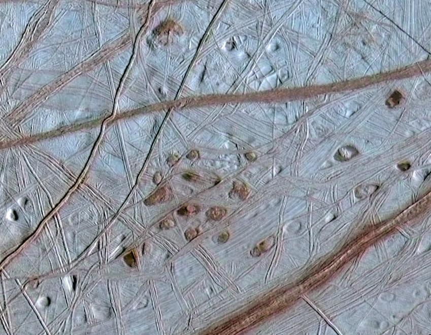
Dark mottled terrain dominates the trailing hemisphere, with ridges and double ridges hundreds of kilometres long being the most ubiquitous landform.  The darker terrains are associated with materials like salts, sulphates, carbonates and/or sulphuric acid on the surface, whereas brighter areas are richer in water ice.  The trailing hemisphere appears brighter, possibly as a result of the more modest particle bombardment compared to the trailing hemisphere.  The main process shaping the surface appears to have been tectonism, with tidal stress (from Europa's 85-hour period for orbiting Jupiter) generating linear ridged plains with dark bands, which subsequently evolved through faulting to create the chaotic terrains at lower latitudes.  However, the mechanisms creating specific features remain highly uncertain, and surface features could be linked to the sub-surface ocean, tidal effects and possible exchange processes.

Only 10% of Europa’s surface was imaged by Galileo at a resolution of better than 100 m, and Europa remains poorly imaged at regional resolutions of 200-500 m.  The highest resolution image obtained by Galileo was at 6m/pixel, revealing the surface to be extremely rough at small scales, but this was only done once.  The JUICE team selected eight regions of interest for their geological, chemical and astrobiological significance, and then designed the flybys to give close views of these locations.  I’ll try to summarise each of those regions below - the Regio, the disrupted terrains, linear features and impact craters.
Regions of interest for JUICE, with the darker
mottled areas known as Regio.  Ground-tracks for the two
flybys are shown. Credit:  ESA Red Book.

1.  Regio:  Darker Terrains:

At low spatial resolution, Europa’s Regio are locations of darker terrain and are given names from Celtic mythology.  On the trailiing side during the approach phases JUICE will be able to observe Annwn (20N, 40E), Argadnel (15S, 151E), Dyfed (10N, 110E), Falga (30N, 150E) and Moytura (50S, 65E) Regio.  On the leading side, JUICE will observe Balgatan (50S, 330E), Powys (0N, 215E) and Tara (10S, 285E) Regio during the departure phases.

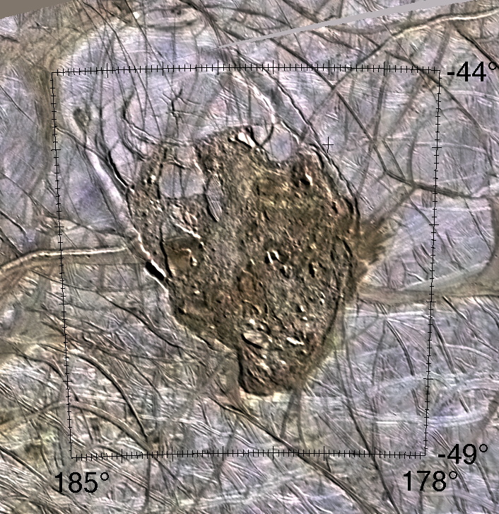
2.  Disrupted Terrain:  Chaos and Lenticulae

Conomara Chaos from Galileo.
Conamara Chaos (A1, 8N, 85E)
Fractured plates of ice that have shifted with respect to one another, possibly due to localised melting of the salty ice shell due to ice convection or oceanic plumes, form the jigsaw of the chaos terrains.  The chaos rafts show pre-existing ridged plains that have been broken up.  Some chaos units appear to stand higher than the surrounding terrain, whereas other appear to have foundered into a finer-grained material.   Reddish material is associated with the chaotic terrain, possibly hinting at a relationship with the deeper ocean.  JUICE will be able to investigate the Conamara Chaos region (A3, 8N, 85E) that has previously been explored by Galileo, but will additionally study chaos terrains in the central and northern parts of the Dyfed Regio region (B1e, B1b, B1c) associated to Conomara, where the activity has disrupted the Asterius, Glaukos, Agave and Belus Linea.

Thera Macula, from Paul Schenk's Atlas of the
Galilean satellites. 
Thera (47S, 179E) and Thrace (46S, 188E) Macula (A3)
These two features, enriched in dark materials potentially emplaced in a liquid state, were considered the highest priority for the flyby.  Thrace is the largest of the Maculae at 180 km diameter, Thera is only 95 km wide.  Here we find chaos material with a matrix of pre-existing structure associated with dark plains, possibly with emplacement of liquid via some sort of cryovolcanism.  Three other Maculae (Boeotia, Castalia and Cyclades) are found in the southern hemisphere (54, 2 and 64S, respectively) around the antijovian point. The inset region of Thrace was imaged by Galileo at 40m per pixel, the rest of the image has a scale of 250m.

Lenticulae (A5, 45N, 145E):
Pits, spots and domes all suggest ice shell convection and are found throughout Europa’s mottled terrain.  These relatively recent circular/elliptical domes and pits (10-15 km across) are associated with prominent intersecting ridges Minos, Udeaus and Cadmus Linea.  Within the domes there is a texture referred to as ‘microchaos’.  Their possible origin is from upwelling of warm, ductile ice, with evidence of melting and exchange with the subsurface.
Lenticulae (Latin for 'freckles') on Europa.  NASA / JPL / University of Arizona / University of Colorado

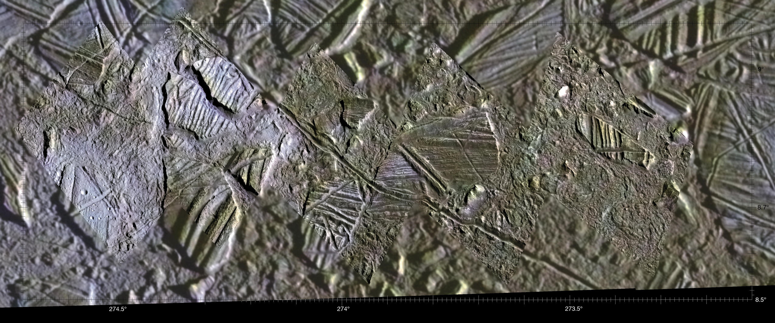
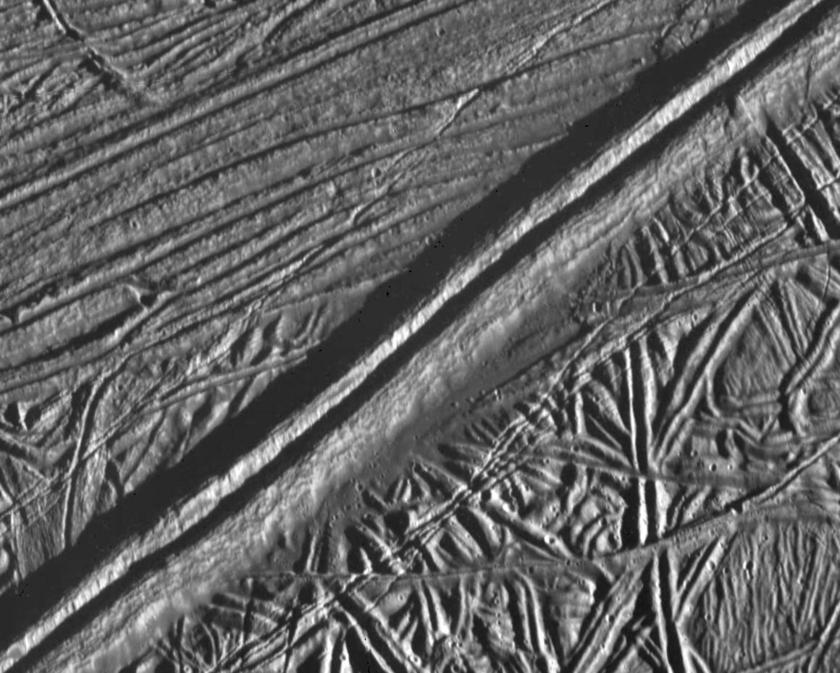
3.  Linear Ridges, Bands and Fractures    

Linear features cross Europa’s surface for hundreds of kilometres, possibly due to fracturing of the icy crust.  Ridges have widths as wide as 2 km and can be several hundred metres high.  Some are double structures separated by a central trough; some are cycloidal and form chains of arcs.

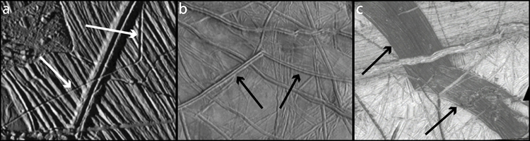
 Three common morphologies of linear features on Europa (a) trough (b) ridge (c) band.  NASA / JPL / Marshall and Kattenhorn

Double ridge on Europa, Feb 1997, NASA / JPL / ASU

Ridged Plains (8S, 140E)
Complex network of ridges, bands and chaos.  Double ridges could form from extrusion or intrusion of water or warm ice, with frictional shear heating from motions (strike-slip faults) along fractures causing warming and melting, creating mobile ice to squeeze through fractures to form the ridge.  Bands could be formed by the pulling apart of the crust by separation and spreading.  

Band Wedges (A6, 5S, 160E):  
These appear to be lineaments that were opened, separated and then filled by a darker (low albedo) non-ice material, much like sea-floor spreading on the Earth.   These wedge-shaped pull-apart bands provide evidence for the original configuration of the ice before the surface began to move.  The youngest bands tend to be the darkest, whereas older bands are bright.

Fractures
Fractures are narrower than the ridges and bands, and are seen down to the 10-m resolution limit of the best images to date.  They can exceed 1000 km in length, cutting across nearly all other features to suggest that deformation of the ice shell occurs over short timescales.  The youngest fractures could even be active today, in response to tidal flexing.

Pwyll crater with bright rays, NASA/JPL/Arizona

4.  Impact features:

Only 24 impact craters larger than 10km in diameter have been identified on Europa, providing strong evidence for a youthful surface.  Taliesin (22S, 222E) is the largest at 50 km diameter, followed by bright Pwyll at 45km diameter.  Multi-ring structures from an impact, can provide information about the physical properties of the sub-surface.  There are very few large craters on the surface, hinting at an age of around 60 million years. Pwyll on the trailing hemisphere (25S, 89E), named for the Celtic god of the underworld, is the most striking of the impact features, and the bright rays suggests it formed less than 5 million years ago.  Pwyll is shallow and relaxed. Multi-ring structures like Tyre (34N, 214E) suggest that the impactor punched through 20-km thick ice, with a central peak from a rebound and surrounded by faulting.


More details of these features can be found in the Gazetteer of Planetary Nomenclature maintained by the USGS:
http://planetarynames.wr.usgs.gov/Page/EUROPA/target

ESA's Europa Flyby Plans

While excitement builds for NASA’s flyby mission for Europa, ESA’s plans for the Jupiter Icy Moons Explorer (JUICE) are now in the implementation phase (known as B2), following successful mission adoption in November 2014.  JUICE will conduct two close flybys of Europa over a couple of weeks in October 2030, before moving onto a wider jovian orbit to complete a reconnaissance of the rest of the jovian system, ending up in orbit around Ganymede in 2032-2033.  JUICE’s sophisticated instrument suite of cameras, spectrometers (UV, near-IR and sub-mm), field and plasma instruments, laser altimeter and sub-surface radar will study Europa’s surface and sub-surface with a clarity, resolution and sensitivity far in excess of any previous exploration, including the ill-fated Galileo mission.  JUICE aims to understand the composition of non-ice material on the surface (particularly those related to habitability of the sub-surface ocean); search for liquid water below the surface; and to study any active processes.

However, the harsh radiation environment of Europa, coupled with the desire to study Jupiter and Ganymede over a 3-year mission, means that JUICE’s brief foray close to Europa will only occur once, with two quick flybys to limit the radiation dose.  Indeed, particle fluxes are 20 times higher at Europa than they are at Ganymede.  We chose to focus these two flybys on regions of high interest for geology, chemistry and astrobiology, including those where Galileo image suggested potential recent activity - chaotic terrains where exchange of materials between the surface and subsurface might have been possible, providing potential insights into the nature of Europa’s subsurface ocean.  Two flybys will no-doubt leave us wanting many more, but it should be remembered that Ganymede is the primary target of this mission.

Regions of interest and trajectory for the two JUICE
flybys of Europa, from the JUICE Definition Study Report.
JUICE will fly on the anti-jovian side of Europa (the far side, from Jupiter’s perspective), with a closest approach of 400 km.  We need to be on the far side for the radar sounding to work.  The far side must also be sunlit for the remote sensing experiments.  This will provide regional (500-1000 m resolution) and local (50 m resolution) imaging for the study of geological processes; the potential for radar sounding down to a maximum penetration depth of 9 km (depending on the surface properties) with a vertical resolution of 50 m or larger; and laser altimetry with a vertical resolution of less than 5 m.

Plans for the Flybys

The spacecraft will approach Europa from the trailing hemisphere (longitude of 90 degrees) that receives the largest radiation dose from the co-rotating jovian magnetosphere; closest approach will be over the anti-jovian point (longitude 180 degrees); and departure is then over the leading hemisphere (longitude 270 degrees).  One flyby will occur over the northern hemisphere (up to latitudes of 45 degrees), the second will be over the southern hemisphere.    JUICE will zip past at 3.6-3.9 km/s.  

The Europa flybys represent the most highly packed observational sequence of the JUICE mission.  Observations will start many hours before the closest approach, using regional imaging and spectroscopic mapping to compare the geology and composition of the leading and trailing hemispheres. JANUS will lead 3 spacecraft slews during the inbound and outbound phases, MAJIS will lead 2, with other instruments riding along to view both the nadir and limb of the moon.   All instruments will be operating simultaneously when the spacecraft is within a distance of 150,000 km of Europa, placing one of the toughest requirements on the design of the JUICE spacecraft.  

During the 2 hours surrounding the closest approach, JUICE will switch from the power-optimised yaw-steering mode to the inertial pointing mode.  After more spacecraft slews, the instruments become purely nadir-pointing for the ±30 minutes around closest approach, and then active instruments (laser altimetry and sub-surface radar) operate for the ±7 minutes surrounding closest approach.  Depending on data volume constraints, distant Europa observations for plume searches will be performed two days either side of the closest approach, and distant views of Europa will continue to be used to study materials ejected from Europa’s surface, such as plume activity from the southern pole.  

Eight regions of interest have been identified, seven of which are on the trailing hemisphere to be viewed during approach.  I’ll try to describe each of these regions in a future blog post, and why we think they’ll be exciting to explore.  The plans continue to be formulated as JUICE moves through the implementation phase, under the guidance of the working groups for the SWT (science working team), but a comprehensive summary of the plans can be found in the JUICE Definition Study Report (Red Book) here:


NASA's Europa Swiss Army Knife

This week at the Applied Physics Laboratory (APL) in Maryland, the Outer Planet Assessment Group (OPAG) is meeting and sharing ideas and progress, and I'm indebted to all those tweeters who contributed to the #OPAG hashtag during the meeting to allow me to write this summary. It also provides an opportunity to discuss the newest of NASA’s missions, the as-yet-unnamed Europa mission.  The mission is expected to perform 45 flybys at altitudes ranging from 25 to 2700 km.  All of the PIs of the selected instruments were present to describe the experiments that will be onboard, described by Bob Pappalardo (mission project scientist) as sending a versatile Swiss Army knife to the outer solar system.  Although this isn’t the orbital mission that we’d originally planned when this was still part of EJSM (the Europa Jupiter System Mission prior to 2010), NASA expects that the flyby mission will still recover 90% of the intended science return.

The mission is now in Phase A, which means that it’s still in flux and being formulated, with many ideas on the table - Hubble is still searching for further evidence of plume activity from Europa’s south pole; potential contributions from ESA are being explored (such as landers, life detection, small free flyers), and about 250 kg of launch mass is being retained from the Phase A studies for more consideration in 2016.  Out of 33 submitted proposals, nine instruments have been selected to explore habitable conditions on Jupiter’s enigmatic moon:

1.  UVS - an ultraviolet spectrograph from Kurt Retherford and colleagues at Southwest Research Institute that’s a clone of the one being flown on ESA’s JUICE spacecraft, which will continue to hunt for plumes from Europa’s subsurface, determine their composition and chemistry, sources and sinks, structure and variability.  It uses a combination of UV emissions, surface reflections and transmissions (e.g., stellar and solar occultations) to detect and characterise Europa’s surface and tenuous atmosphere.

2.  EIS - the Europa dual imaging camera system led by Zibi Turtle of APL, combining both a narrow (NAC) and wide angle camera (WAC) with colour and stereo capabilities to understand the formation of landforms, the potential for current activity on the surface, and characterise the ice shell and ice-ocean interface.  The NAC has a 2-axis gimbal that allows the FOV to be moved both within and beyond the field of the WAC, achieving resolutions of 0.5 m from an altitude of 50 km above Europa’s surface.  The WAC will have a resolution of 4m from 50 km altitude, over a wider surface area.  The whole surface of the moon could potentially be mapped at a resolution of 50m.  The stereo capabilities will allow the creation of a digital terrain model (DTM) with a 4m vertical precision from the 50-km flyby altitude.  

3.  MISE - the mapping infrared spectrometer for Europa led by Diana Blaney (JPL) will be used to map the history of geologic activity on the surface, including a search for currently active areas.  Covering 0.8-5.0 µm with a 10 nm spectral resolution, this near-infrared spectrometer is a common feature of missions - Cassini, Juno and JUICE all have similar experiments (VIMS, JIRAM and MAJIS).  MISE will get resolutions of 25 m on a local scale, 300 m on a regional scale, and 10 km on a global scale, assuming 100-km altitude flybys.  Near-IR reflectance spectra will allow distinguishing between hydrate regions, sulphate regions, and even search for trace organics.

4.  E-THEMIS is the thermal instrument on board (so glad NASA chose to take a mid-infrared instrument, and I wish ESA/JUICE had one too!), provided by Phil Christensen of Arizonal State University.  The instrument will search for thermal anomalies on the surface (particular associated with any active venting), with a resolution of 5x22 m from 25 km altitude and a precision of 0.2 K for 90-K surfaces and 0.1 K for 220-K surfaces.  It has three filters, 7-14, 14-28 and 28-70 µm.

5.  REASON - the Radar for Europe Assessment and Sounding: Ocean to Near-Surface provided by Don Blankenship and team at Texas (best acronym ever), and a sister instrument for the RIME instrument on ESA/JUICE.  It’s a dual frequency radar at 60 MHz, with 15-m vertical resolution for shallow sounding to 4.5 km depth, or 150-m vertical resolution for ocean sounding below 4.5-km depth.  It will study the surface, sub-surface, using reflectometry to study near-surface roughness, porosity and composition, and search for an ice-ocean interface and evidence of exchange processes beneath Europa’s surface.  

6. PIMS - the plasma instrument for magnetic sounding provided by Joe Westlake from Johns Hopkins APL, which will work to characterise the salinity and depth of Europa’s oceans by measuring the plasma environment surrounding Europa and the magnetic induction response as conductive Europa moves through Jupiter’s magnetosphere.

7.  ICEMAG - the mission magnetometer provided by Carol Raymond of JPL to characterise Europa’s interior, thermal evolution, atmospheric sources and sinks, and the coupling between Europa and Jupiter’s ionosphere.  ICEMAG can also look at Europa’s exosphere by looking at dynamic species coming off Europa during each flyby.  

8.  MASPEX - a mass spectrometer provided by Hunter Waite and colleagues at the Southwest Research Institute (SwRI) to sniff out the exospheric (and ejected surface) composition.  Particles can be sputtered from Europa’s surface due to bombardment by energetic particles, or can simply sublimate from the surface, creating a density enhancement over the sunlit region.  Plume material would also contribute, being transported equatorward and deposited at lower latitudes to join other materials to be sputtered.

9.  SUDA - a dust experiment to characterise the surface using lofted dust detected with low-altitude flyby, provided by Sascha Kempf of University of Colorado, Boulder.  The Galileo dust detector had previously found that each of the Galilean satellites were wrapped in dust clouds of surface ejecta.  euro

More information on each of these instruments can be found here:
…and I’ll try to compare the capabilities of the Europa mission to those of JUICE (which will be performing two Europa flybys) in future blog posts.


Monday 27 July 2015

The Problem with Earth 2.0

Like many others, I'm starting to develop a severe twitch whenever I see the words 'Earth-like' or 'Earth twin' or 'Earth-2.0'.  The twitch was pretty maddening last Friday, when the the discovery of Kepler-452b was announced by NASA and shared globally by media outlets, including the BBC report here.  The paper, by Jenkins et al. (arxiv), describes the detection of a "possibly rocky" world 1.63±0.2 times the radius of Earth, orbiting a Sun-like star on a 385-day orbit.  In fact, the probability of this world being rocky lies somewhere between 49% and 62%, according to models and their statistical analyses.  So it's a 50:50 chance of being a rocky world.  The star is slightly older and larger than our own Sun, and at 1400 light years from Earth it's going to be an immense challenge to learn more about the conditions on this world.
Stunning artists impression of newly-discovered Kepler-452b.
But we should recognise the artist license here, and that these
works don't begin to portray the uncertainty!

Taking a step back for a moment, the very fact that our species has been able to build machines that today, in the early 21st century, are capable of discovering worlds that *could* be similar to our own is pretty breathtaking - an incredible feat of human achievement that we hope has been matched and exceeded by other civilisations out there in our universe!  Exoplanetary science has advanced at an incredible rate, with understandable excitement surrounding new discoveries and what these new worlds might be like.  The problem is that our excitement is sometimes overreaching what we truly know about these distant worlds.  Sadly, the answer to that is "next to nothing."

The paper by Jenkins and the Kepler team is very clear about this.  They write about probabilities and present the facts, as scientists should be doing.  There are subtleties and complexities in the reduction and interpretation of these data that could take years to fully understand, and science is honest about all this. The problem is that the media, by and large, are after a catchy headline to make us buy their papers or click on their ads. And public outreach departments for universities, businesses and space agencies all know this.  This chain means those subtleties are lost, and we're left with headlines about the discovery of an Earth twin.  And it's that which drives so many of us nuts.

The problem is that the community starts to look like the 'boy who cried wolf.'  Yes, we're now another step closer to the goal of finding an Earth (in this case, we know so little about this world that it could be rocky, but it could also be gassy and very unlike our home).  And yes, this could be the closest we know of to date.  But with every step, these big media releases diminish the next discovery.  Media outlets will work harder and harder to push their headlines, using more and more hyperbole to describe the new results.  Eventually, will people care when a true Earth twin is discovered by some future telescope?  As scientists on Twitter have pointed out, this regular news headline is becoming as familiar as the story of water on Mars ("yawn, we've discovered evidence of Martian water.... again...").  And one day, will we be saying "scientists have discovered more biomarkers in exoplanet BLAH756b's atmosphere... yawn...", because of this need to publicise work to win public admiration and sorely-needed grant money?

I'm being mean, as I've publicised things that didn't need publicising, so I can understand the temptation.  And there's the flipside - some budding young wannabe scientist might see this news and think "that's what I want to do with my life."  And that'd be a great thing.  I hope it prompts them to look deeper, follow through the hyped-up press releases and actually read the scientists' words directly.  It's what we don't know that's keeping the community so excited about these new discoveries!  What about its atmosphere? Magnetic field?  Plate tectonics?  Oceans and mountains and vegetation and life?  What if it's a small version of Neptune?  That's what get's me fired up.

PS.  Read Phil Plait's take on all this here.


Monday 20 July 2015

Airbus DS Selected for JUICE

Seven months after the announcement that the JUICE mission had been formally adopted by ESA (November 2014), and the Invitation to Tender (ITT) released to the prospective contractors in December, we learned last week that Airbus Defence and Space (@AirbusDS) has been chosen by ESA's Industrial Policy Committee to build our ride to the jovian system.  The selection of an industrial contractor is making the whole process feel so much more real, and Airbus is expected to sign the contract in September.  That means that work could start as early as the end of the month.

Airbus DS is "the world's second largest space company," with sites around Europe in Toulouse (France), Friedrichshafen (Germany), Stevenage (UK) and Madrid (Spain).  They're very well known in planetary exploration, having built Venus and Mars Express, Huygens for Titan and the Rosetta spacecraft.  Today they're building ExoMars, BepiColombo and Solar Orbiter, so with that heritage they seem like a great choice to me.  Building the 5-tonne JUICE spacecraft will be a challenge, with its 97 square metres of solar panels to provide the juice for JUICE out at 5AU, and the requirements for an unprecedented level of magnetic cleanliness to prevent any problems with the sophisticated payload suite.

Airbus DS won the €350M contract ($389M) after a competition with a team composed of Thales Alenia Space of France and Italy and OHB SE of Germany.  From ESA:  "The contract covers the industrial activities for the design, development, integration, test, launch campaign, and in-space commissioning of the spacecraft. The Ariane 5 launch is not included and will be procured later from Arianespace."

From spacenews:  "ESA’s geographic return rules mean work-share distribution must closely match each nation’s financial input, meaning Germany, France, Britain and Italy, as ESA’s biggest members, must be guarantee major pro rata roles for their domestic industry."  That means the the individual ESA member states must get out what they put in, so everyone will hopefully get a slice of the JUICE pie...

Read ESA's press release here and Airbus' release here.

Monday 6 July 2015

Latex Papers Survival Guide

Every now and then I spend hours of my time wrestling with Latex documents to get them to do my bidding.  I'll try to keep a record of any useful hints and tips here.

Text Highlighting:

To highlight paragraphs of text, including references:

\usepackage{color,soul}

...and then when you get to the text you want to highlight, simply add \hl{...}.  To ensure that references behave properly when using the \cite{} suite, put it inside an \mbox{} command.  I.e., use \mbox{\citep[][]{87andrews}}.


Friday 26 June 2015

IUGG and Planetary Meeting Overload

I’m in the air returning from a relatively poorly-known meeting in planetary science, the IUGG (International Union of Geodesy and Geophysics, http://www.iugg.org/) meeting that was held this year in Prague.  These quadrennial meetings have an extremely long history, dating back to 1919 when they were first established in Brussels, but they are mainly dedicated to studies of planet Earth and its immediate environment.  There’s a smattering of ‘off-world’ topics scattered throughout the Union’s remit, but the number of Earth scientists engaging with their planetary science counterparts is relatively low.  I hope that will change, and this year myself and others convened a couple of comparative planetology sessions, hoping to attract a broad audience from across IUGG.

IUGG is one of the 31 Unions that make up the International Council of Science (ICS, http://www.icsu.org/), which also features the IAU (International Astronomy Union), famed for its demotion of Pluto from planet status.  These Unions are organised in very specific ways - the IUGG has eight Scientific Associations (cryospheric science, geomagnetism and aeronomy, meteorology and atmospheric science, seismology and Earth’s interior, geodesy, hydrological science, ocean science and volcanic science).  Each Association then has a number of commissions that operate on a more detailed level.

Within IAMAS, the International Association of Meteorology and Atmospheric Sciences (http://www.iamas.org/), I have been helping to manage one such commission, known as the International Commission for Planetary Atmospheres and their Evolution (ICPAE).  I’ve been the Vice President since my election in 2011, with Sanjay Limaye (University of Madison Wisconsin) as the President.  After four years I’ve decided to step down due to other commitments, but I wanted to record here my understanding of how all of these Councils, Unions, Associations and Commissions are organised.  To a newcomer, all the acronyms can be mind-boggling.  The next meeting in 2017 is known as the IAGA-IAMAS-IAPSO meeting, for example, which doesn’t tell you very much!

I certainly like the idea of these international unions and associations - these meetings are among the most diverse that I’ve ever attended, with people from all over the world attending.  So collaborations are clearly being fostered, but in the planetary community, straddling both the astronomical communities and the geophysical communities, we’re swamped with a ridiculously high number of meetings.  On a continental level there’s AGU (American Geophysical Union), AAS (American Astronomical Society) and DPS (Division of Planetary Sciences) meetings in the US; EGU (European Geophysical Union) and EPSC (European Planetary Sciences Congress) in Europe; AOGS (Asia-Oceana Geophysical Society) in Asia, and many more meetings at a national level.  Then there are ‘international’ meetings like COSPAR (Committee for Space Research, https://cosparhq.cnes.fr/), which is actually also a part of the International Council for Science (ICS…. and the acronym forest grows thicker), and newcomers like ExoClimes and the Chapman meetings…. the list grows every year, and I sometimes groan when new meetings are announced.

All in all, you never find the whole planetary community at one single meeting.  Each meeting has it’s own problems (too many parallel sessions, expensive locations, etc), and although DPS and EPSC are my personal favourites, it’s hard to keep up with the constant calls for abstracts. Even harder when dealing with funding councils who don’t always recognise that travel is essential for collaboration and ‘selling’ your science!  One look at the gargantuan multi-page tables of acronyms that made up the IUGG conference program confirmed that I’d made the right decision.  For me, the IUGG meeting was a good example of conference overload, with only a few tens of planetary scientists attending, despite the great opportunity to meet with our Earth science colleagues.  Hopefully the 2017 meeting can be made more inclusive to attract a wider audience.

Sunday 8 March 2015

The Atacama Large Millimetre/Sub-Millimetre Array (ALMA)

Our flight to northern Chile and stay in San Pedro de Atacama was designed so we could acclimatise to the high altitude and arid conditions of the high desert before visiting the radio observatory at 5050 m on the Atacama plateau.  ALMA is the world’s most sophisticated observatory at these wavelengths, a truly collaborative project between Europe, Japan, America and Chile.  It works by having fifty 12-m antennae (the Main Array) with variable separations in between.  The different baselines allow you to take a Fourier Transform of the sky, correlating the signals from each antenna to provide a spatial resolution far superior to what you can achieve from a single dish in isolation.  The sensitivity to a particular spatial scale depends on the length of the baseline.  Short baseline configurations (150-m) provide access to large spatial scales; long baselines (up to 15 km) provide access to the smallest spatial scales. Twelve additional 7-m antennae (the Compact Array) provide very short baselines for the largest spatial scales.

Within each antenna is a series of receivers, or bands, which determine what wavelengths can be observed.  At the moment bands 3-9 are available to users, providing wavelengths from 420 µm to 3.6 mm (84-720 GHz).  This should extend up the 950 GHz when band 10 is offered, and maybe down to 30 GHz with future receiver development.  Measurements in these spectral bands, at a variety of spectral resolutions, are then fed by cables to the main correlator building a few metres away from the antennae, using the Fourier Transform to assemble an image of the sky with unprecedented spatial resolution.


The ALMA site offers the best observing conditions in Chilean winter (July to November), so the more challenging configurations are used then.  In February the conditions are usually hazardous with extreme snowfall, meaning that the antennae must be oriented so that snow does not accumulate inside the dishes.  Conditions below the snow line can be so wet that flash flooding can destroy the access roads.  Thankfully, by the time of our visit in March, conditions were cold and clear again and excellent for some astronomy tourism.

Extreme Tourism at 5 km 


On Saturday morning we met a bus at 7am for the drive out to the OSF (Observer Support Facility) at an altitude of 2500m.  The sun was rising over the volcano to the east as we drove the dirt road to the facility, a cluster of buildings featuring the main control room and data banks, in addition to the hangers and workspaces of the contractors from Japan, the US and Europe responsible for constructing and delivering the 66 antennae (now empty as their work is done).  Construction was still taking place for a permanent visitor quarters, with temporary buildings housing the astronomers.  We had to each undergo a compulsory medical exam (blood pressure and O2 levels) and safety video, being supplied with small oxygen canisters to use should we feel dizzy at high altitude.  This is a serious medical screening - one of our number didn’t pass and had to remain at the OSF.

We ascended the switch-backed road through the mountains, watching as the dry slopes gave way to some green vegetation and cacti, allowing the grazing donkeys and llama (vicuna) to survive despite the seemingly hostile conditions.  The landscape was not as volcanic or young as that on Mauna Kea, this is a more ancient geology.  We all started to feel lightheaded, but cheered as we passed the 4200-m mark (the height of the Mauna Kea observatories).  For many of us, this marked the highest point we’ve ever been to in our lives.  As we crossed the mountain pass, the plateau opened up before us and the ALMA array came into view.  A small Japanese observatory could be seen on one of the high peaks, which must be one of the highest manned observatories in the world.

We had about half an hour to wander amongst the antennae, which was in a compact configuration after the February snows and undergoing engineering work to prepare for more science.  Eric Villard served as an excellent tour guide, showing the differences between the US and European antennae designs.  As we watched, one of the antennae rotated around silently, controlled by some unseen operator down at the OSF.  The thin air (0.5 bar) and lack of O2 at 5050 metres above sea level does strange things to the brain, an almost drunken experience as we posed for photos with the array in the background.  All of us took occasional puffs from the oxygen canisters if we felt any dizziness, but thankfully I didn’t experience any of the headaches or nausea sometimes associated with high altitude.

We then went inside the correlator building, seeing the banks and banks of computers and hard drives required to bring together the signals from each of the individual antennae.  Then it was time to begin our 45 minute descent back to the OSF for lunch and then on to Calama, drinking in the thicker atmosphere and feeling tired.  It had been a tremendous experience, not only because I now know more about the challenge of radio interferometry for astronomy, but also because of the extreme environment we’d been lucky enough to visit.  Very few humans get this opportunity, so I’m extremely grateful to ESO and the organisers of #planets2015 for the chance!

Friday 6 March 2015

San Pedro de Atacama

The planetary science workshop ended on Thursday evening, but eighteen of us stayed on in Chile with the opportunity to visit the Atacama Large Millimetre/Sub-Millimetre array (ALMA), high in the Atacama desert in northern Chile.  This was a chance not to be missed, both for the otherworldly environment and the prospect of glimpsing the worlds most sophisticated radio observatory.

We departed Santiago for the two hour flight to Calama, cruising to the west of the Andes and passing the tallest peak in the whole of South America (Aconcagua), 7000 m high and in neighbouring Argentina.  The landscape below was dry and desolate, punctuated by extensive mining works for copper and lithium (apparently Chile is one of the largest global exporters of lithium, making money out of its use in electronics all over the world).  The Atacama is the world’s driest non-polar desert, with some rain gauges having never received any rain, period.  And you could really tell from the air.  Calama itself was a dust bowl, and the rich salt lakes covered the land right up to the mountains (extinct and ancient volcanoes).

A 90-minute bus took us from Calama to San Pedro de Atacama, a small town grown around an oasis in the desert.  We passed through the study Valle de la Luna, with sedimentary rocks thrust and turned on their side to produce a vast red canyon of jutting rock formations.  San Pedro was a really striking experience, as every building was made of the red-coloured adobe, including our hotel the Casa de Don Thomas.  The streets were largely unpaved and prone to dusty breezes flowing through, stray (but not aggressive) dogs roamed everywhere, and waterways criss-crossed the town for use in irrigation.  The village had a central square, featuring an adobe church that was undergoing renovation, a museum containing archaeological remains of the Chilean peoples who first lived here, and a relaxed bar with tables spilling into the square.  There’s one long main street, featuring endless small restaurants, souvenir shops and excursion organisers (from here tourists can visit a geyser field, salt lakes, flamingo reserves, or go sand boarding).

Sadly I had no time to enjoy the resort, only having a couple of hours to stroll the main street and dine in the Adobe restaurant.  Others stayed on for a few extra days following our trip to ALMA, but for me it was time to leave Chile behind.  I returned to Santiago on Saturday night for a brief stay in an airport hotel, then an early morning flight back to London via Sao Paolo.  Incidentally, the 4-hour stop in Sao Paolo on the Tropic of Capricorn was my first ever trip to Brazil!  One day I’ll have to come back….

Thursday 5 March 2015

ESO Planetary Sciences Workshop 2015

The purpose of my visit to Santiago this spring was to present an invited talk at the ESO “Planets 2015” workshop, known as a “Joint Venture in Planetary Science” between space-based and ground-based observatories.  Organised by Eric Villard (ESO and ALMA) and Olivier Witasse (ESA, and the new project scientist for JUICE), this meeting brought around 80 planetary scientists together for four days in the ESO Vitacura office.  It was a wonderful opportunity to meet people and forge new collaborations, and certainly one of the best meetings I’ve been to in a long time.  Several of us were live-tweeting the meeting, so the highlights can be found there, or via this link on storify.

Science Sessions

Following a keynote talk by Mike Mumma from Goddard Center for Astrobiology, the days were subdivided into science sessions and facility sessions, punctuated by healthy coffee breaks and lunch sessions sat in the gardens surrounding the ESO office.  Monday covered giant planets, where I delivered an overview talk on synergistic studies of dynamics, chemistry and origins from spacecraft and telescopes (I’ll try to summarise that at some point), Imke de Pater revealed gorgeous VLA images of Jupiter; Gordy Bjoraker showed high-resolution 5-µm spectra of Jupiter and Saturn; and Ted Kostiuk gave an overview of atmosphere-auroral interconnections via infrared spectroscopy.  Tuesday’s science session covered terrestrial planet atmospheres (including a Doppler velocimetry technique to measure winds using visible spectroscopy), focussing on Venus and Mars, but with some fascinating ALMA results on Titan (Cordiner) and Io (Moulet), and Katherine de Kleer’s long-term program to monitor Io’s volcanic activity in the L and M band (3-5 µm) using Keck and Gemini.


On Wednesday we venerated into the realm of asteroids, TNOs and comets, including radar observations of asteroids where Benner produced 3-D printed versions of asteroid Bennu (the destination for the OSIRIS-REx mission, due to launch in the next couple of years) showing an equatorial bulge and distinct ‘boulder’ on the surface.  We heard about the jovian trojans and hildas, asteroid families that I know very little about; the discoveries of rings around the centaurs (Chariklo and Chiron); and the prospects for detailed studies of Trans-Neptunian objects.  I learned that many of the Kuiper Belt objects featured small satellites, whose names were completely new to me.  Finally, on Thursday we ventured briefly into exoplanets and planetary formation.  The science sessions had covered a very wide range, and I felt I learned the most from the review/overview presentations rather than the more detailed science talks.  If this meeting were to happen again, a stronger emphasis on review and forward thinking, rather than focussing on your own research, might be the way to go.

Facility Sessions

In contrast, I got a lot more out of the four facility sessions.  As we were sat listening to the presentations on the various observatories, I could see many people in the audience thinking of new ways to study their fields, me included.  Monday afternoon served to pique my curiosity about ALMA, as Eric Villard presented the capabilities of ALMA for planetary science (more on that in a later blog post).  We heard talks on:


  •    The Mauna Kea sub-millimetre valley (SMA, JCMT and CSO) by Mark Gurwell; 
  •    Eliot Young reviewed NASA’s ideas for balloon-borne planetary observatories;
  •    The US NRAO (National Radio Astronomy Observatory) facilities, including the VLA, VLBA and Green Bank Telescope (Butler);
  •    The SOFIA observatory and its instrument suite (Reach);
  •    Ground-based support for Cassini and Juno (Orton);
  •    Use of the deep space network for both telemetry and science via radio link (Lasio);
  •    Instrumentation roadmaps and plans for the Paranal observatory (VLT) in contrast to Keck and Gemini (Dumas);
  •    Plans for the NASA Infrared Telescope Facility (Tokunaga);
  •    The capabilities of the Large Binocular Telescope and Interferometer (LBTI) for high angular resolution studies (Conrad);
  •    IRAM for millimetre studies (Boissier);
  •    The prospects for the James Webb Space Telescope (JWST) for solar system science (Stansberry).


Having experts in these facilities in the same room as the science users proved to be an excellent idea. I had so many useful discussions over coffee and lunch that my to-do list is now enormous.  ALMA, although heavily oversubscribed, is particularly exciting and it would be great to use it for giant planet science.  I got to talk to the instrument scientists in charge of the VISIR renovation and recommissioning (a work-horse of mine for infrared imaging and spectroscopy) and hopefully instilled an excitement for looking at Jupiter and Saturn soon (time awarded in the next semester).  I discussed our SOFIA/FORCAST data on Jupiter with SOFIA specialists, which we’ll use to study deep circulations.  I met with Japanese colleagues working on Subaru/COMICS Saturn imaging (which I actually acquired, along with Glenn Orton, from the summit of Mauna Kea in January 2008), investigating the changing brightness of Saturn’s rings as a function of season.  I met others working on VLT/SPHERE observations and struggling (as I am) with data reduction.  I caught up with a colleague working on exoplanet observations (who just happened to be in Santiago on his way to the VLT), and with colleagues working on Cassini/CIRS, and had lengthy discussions about organisation for ground-based supporting observations for the Juno mission.  On that topic, one of my first tasks when I get back to Oxford is to draft a white paper to try to convince observatories to support this mission.

The last day of the meeting featured a talk from Will Grundy on the New Horizons mission, particularly the heroic ground-based efforts from John Spencer and other to identify a suitable KBO target for a second flyby after Pluto.  Two candidates were found (PT1 and PT3), ultimately using lots of Hubble time.  But the idea that the Pluto encounter is already underway, and that this whole system will be gradually revealed in glorious detail over the next few months, is breathtaking.  History in the making, and a great way to end the meeting.

Monday 2 March 2015

Santiago de Chile

I’m back on the road again, but this time for a pretty exciting trip - my first ever excursion to South America, travelling to Santiago, Chile as an invited speaker at ESO’s Planetary Science workshop.  This four-day event is intended to explore scientific overlaps between ground-based observatories and spacecraft exploring our solar system, so it was very easy to say yes to the invitation.  At the end of the week, several of us are flying to San Pedro de Atacama for a trip to ALMA, which promises to be a highlight of the trip.  I’ll be talking on Monday (Day One) about synergistic investigations of giant planet dynamics and chemistry (touching on planetary impacts, storms and global circulation), but I need to get there first.

Flight to Santiago

The trip to Chile involves an evening departure from London, a couple of hour hop over to Madrid, before catching a packed Iberia flight direct to Santiago.  I’m told it’s almost always an overnight flight from Europe, a trip of 6500 miles and 12.5 hours from 52N to 33S, landing in the early morning.  Santiago is the Chilean capital, nested between the Andes to the east and the coastal cordillera to the west, on the Panamericana highway.  My first view of the Andes came as we descended into the early morning Santiago, snow-capped despite the 30-degree summer temperatures of early March.  Escaping the airport was an ordeal - hundreds of people cram into the arrivals hall, screaming ‘Taxi taxi’ at you.  I’ve heard many horror stories of people being ripped off at this point (indeed, some of my colleagues accepted a ride only to wait hours for the van to show up), but I’d been advised to seek out one company, Transvip, to get me to ESO.  They were even expecting me, which made life much easier.

Vitacura

The taxi wound its way from the airport west of the city, spending a long time in extensive underground tunnels before emerging in the shiny and modern Vitacura district to the northeast of the city centre.  Sometimes referred to as ‘Sanhatten’ for its upmarket hotels, skyscrapers and restaurants, this is the home of ESO’s Vitacura office, next to the bicentennial park (Chile declared independence from Spain in 1810).  I stayed in the Hotel Director, along with may of the other conference participants, and we dined every night in various restaurants around the Alonso de Córdova.  I’ve never been been to a conference where I’ve eaten so consistently well every evening, with memorable locations including al fresco dining on fresh sea bass and seafood salad, and the Noi Hotel’s rooftop bar, where we drank pisco sours and Krass beer while the (upside) moon rose over the Andes.  Being with a bunch of astronomers, we spent most of the evening gazing upwards to the southern constellations, and remarking how strange Orion looked from the southern hemisphere perspective.

Exploring Centro and Santa Lucia Hill - Sunday

Given the packed conference schedule, I decided to go exploring in central Santiago on Sunday afternoon, despite the lack of sleep on my overnight flight.  A 30-minute walk down Av. Vitacura took be to the Tobalaba metro station, where I used my finest Spanish to figure out how to buy the ‘Bip!’ card to use the metro system.  Centro was 7 stops and 2 changes away from Vitacura, but it took no time at all and I emerged on the Plaza de Armas to explore the 19th century buildings and squares.  The Plaza is the heart of the city, containing hundreds of palm trees and bordered by the Catedral Metropolitana, built between 1748 and 1800.  I explored the Cathedral, including the subterranean crypt where former bishops are buried, and wandered north to the Mercado Central fish market, a bustling combination of smelly fish stalls and crowded eateries.  The pedestrian streets were packed with sunday-afternoon shoppers, and the whole place felt vibrant and friendly.

I strolled south east through the Centro district to find the Cerro Santa Lucia, a rocky hill that was transformed in the 19th century into a landscaped park laced with trails and steep stairs to reach the summit.  I climbed through the flowery gardens to fine Torre Mirador, a red brick tower at the hilltop providing excellent views of the surrounding city, including a view back towards ‘Sanhatten’ and the snowcapped Andes in the distance.  With that, it was time to descend to the Santa Lucia metro station and return to Vitacura in time for the conference welcoming reception (and a few pisco sours) at the ESO Vitacura office.

With all this exploring, I couldn’t figure out why my sense of direction was so screwed up, until it hit me.  The sun is in the wrong place.  This simple realisation made me laugh out loud - my northern-biased brain is so hardwired to use the sun’s southerly position to allow me to navigate, that the sudden shift into the southern hemisphere completely messed up my internal compass!

Tarapaca Vineyard - Wednesday

Our conference dinner was organised in the gorgeous surrounds of the Tarapaca winery in the Maipo Valley.  Nestled amongst the vines was a small hotel, with rooms named for the grape varieties grown there. We were given a tour of the fermentation plant and wine cellar, and stood  beneath the trees to sample various varieties including a rather tasty carmenere.  After presentations from NASA and ESA representatives on their hopes for greater collaborations between space and ground-based facilities, dinner was a vast barbecue served in the grounds.

Cerro San Cristóbal and Barrio Bellavista - Thursday

I managed to get back into Santiago on Thursday evening, using expensive taxis (we were ripped off by the Hotel) to reach Barrio Bellavista to ride the funicular railway to to the top of San Cristobal hill.  A 14m-high statue of the Virgen de la Inmaculada Concepción sits at the top of the hill, overlooking the city below, and an easy climb from the railway station provided great views in all directions around the city.  In the evening light Santiago is a very hazy place, apparently due to the fact that the city sits in a basin between mountain ranges, and with no sea breeze to clear out the smog.  The Andes could just be seen in the distance, although photographs didn’t really do them justice.

A stroll down Pio Nono brought us past endless lines of noisy bars, filled with students from the nearby university.  Searching for food in the Barrio, we stumbled across the Patio Bellavista, a courtyard of upmarket eateries, and I ate lamb shank drizzled in a syrah and smoked bacon sauce, a superb end to our brief excursion to Santiago.